 HOBI Labs' backscattering instruments feature
HOBI Labs' backscattering calibration method is also integral to these instrument's performance.
The diagram at right shows the basic geometry of the measurement, in cross section. An LED produces a beam of light emerging at an angle from the sensor face. A receiver, whose field of view is tilted at a similar angle, detects light scattered out of the sensing volume within the appropriate range of angles. The crossing angle between the source and receiver defines a nominal scattering angle of 140°.
Backscattering is a very weak phenomenon over small distances. In the HydroScats, the fraction of light backscattered from the sampling volume is only about
10-8! Nevertheless careful electronic and optical design allow the HydroScats to confidently measure the backscattering of
pure water.
In the electronics, selection of components, circuit board layout, switching frequencies, grounding topology, and power supply noise must be carefully controlled. In the HydroScats, electronic noise is essentially at its theoretical minimum: the thermal noise of the first-stage feedback resistor. In conditions of high background light, this noise factor may be exceeded by the shot noise of the light itself.
The optical design also involves many tradeoffs. Among the most important optical parameters are sizes of the aperture and detector. In each case, larger size translates directly into greater light-gathering. Greater angular field of view also helps light-gathering power, but may disproportionately emphasize undesirable background light. The HydroScat optics therefore include large detectors and optical aperture, but narrow angular FOV.
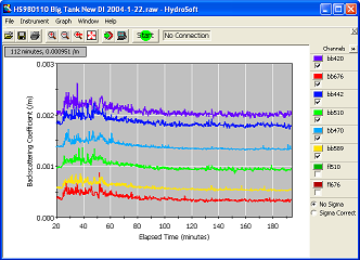
Backscattering vs Time in filtered water
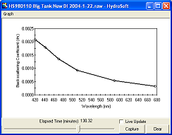
Backscattering spectrum from above;
The plots at right (screens from HydroSoft) show results of an experiment in highly filtered, degassed and deionized water. The first plot shows the six backscattering values over a period of about 3 hours. The elevated noise near the beginning was due to contamination being flushed out of the tank's recirculation pump when it was first turned on. The scattering values gradually declined as the recirculation pump and filters had their intended effect. Eventually the scattering reached values very close to those expected for pure water. The lower plot on the right shows the scattering spectrum near the end of the time series.
These data not only demonstrate the instruments' sensitivity, but also confirm the effectiveness of their calibration.
Like sensitivity, background rejection is controlled by both electronics and opticals. In the electronics, high-frequency modulation, synchronous detection, and bandwidth control in the front end all act to reject constant background as well as wave-modulated light. To cope with extreme conditions, such as operation over a bright sandy bottom, the instruments monitor the background radiance and automatically reduce their gain if necessary.
The small angular field of view of the HydroScat optics helps limit background response, while the large aperture enhances desirable signal response.
Each backscattering channel's signal amplifier has 5 electronically-selectable gain settings, spaced approximately in decades. In combination with 16-bit A/D conversion, this allows them to measure anything from pure water, with its effective reflectivity of 10
-8, to a 99% reflecting plate (as is used during calibration). By default they automatically adjust their gains as appropriate to
in-situ conditions.
Each backscattering LED is constantly monitored by a reference photodiode, spectrally filtered to match the signal bandwidth. The reference measurements are applied within the instrument to compensate for temperature- and age-related changes in LED output. For example, the output power of some LEDs varies by 2% or more per degree of temperature change?as much as 60% over the total operating temperature range. LED output also decreases gradually with time, at rates that vary from unit to unit. Reference compensation reduces all these variations by a factor of 10 or more.
Back to top